Environmental Monitoring Network Planning

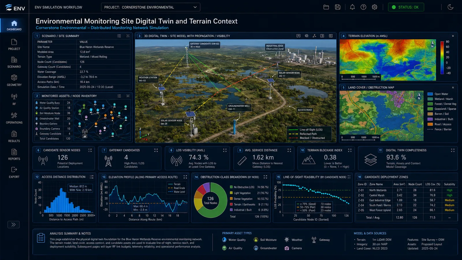
The digital twin stage establishes the geometry that every subsequent stage depends on: terrain, vegetation, water boundaries, retention ponds, groundwater wells, berms, access roads, industrial structures, and the candidate locations where sensors, gateways, and solar infrastructure can plausibly be installed.

This stage answers whether the site supports remote monitoring at all, where elevation, vegetation, water, and access constraints rule out placement, which zones look viable for sensors, and which look viable for gateways. Without it, RF and telemetry analysis quickly becomes detached from field reality.

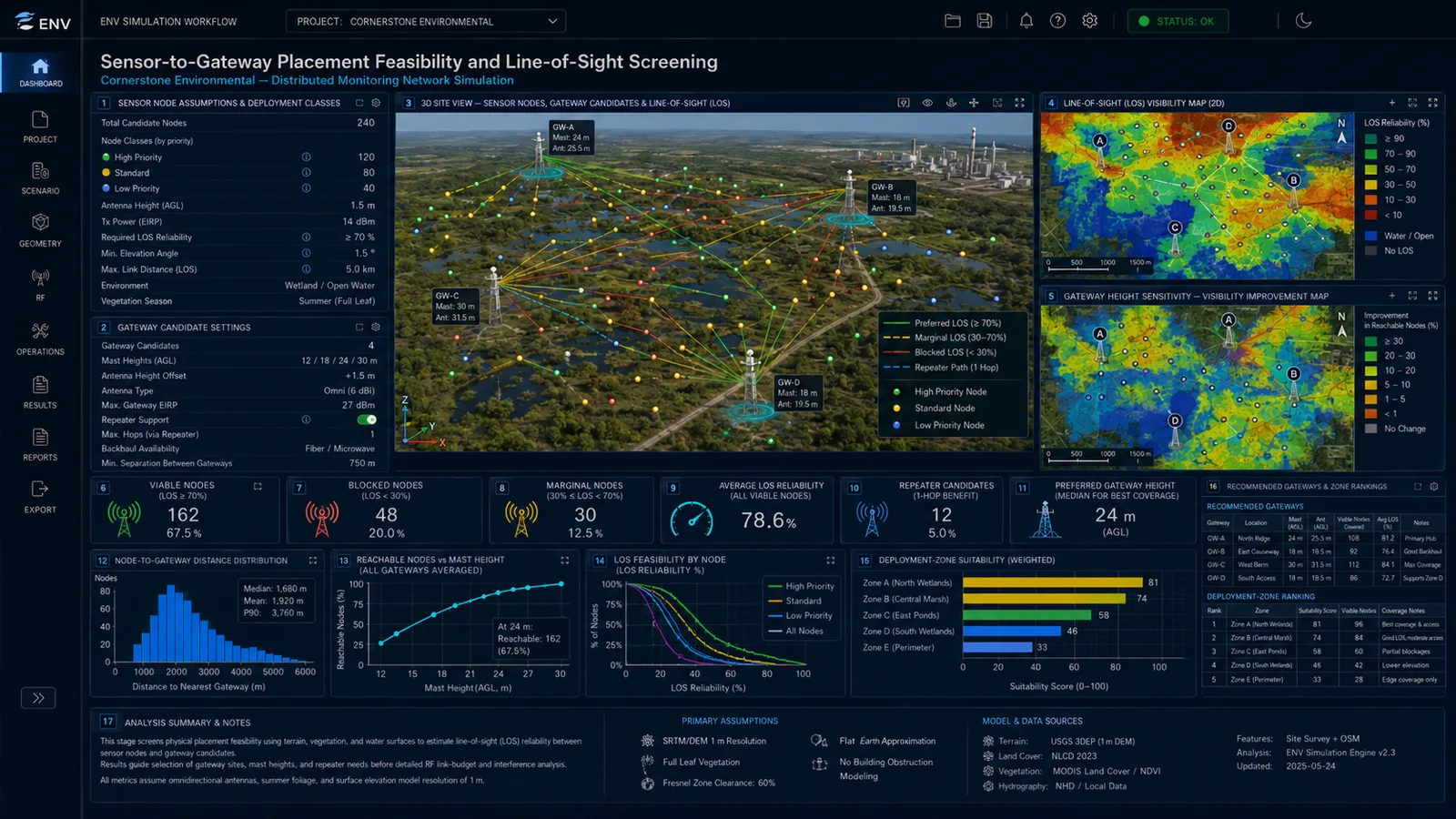
The placement feasibility stage evaluates whether candidate sensor nodes can plausibly reach candidate gateways. It tests line-of-sight, partial obstruction, antenna height, mast height, repeater options, cabinet placement, and physical service access. It does not yet attempt full propagation. Its job is to screen layouts.

This stage answers which sensor sites have a viable path to which gateway, which sites are blocked or marginal, what gateway height is needed to reach the network, where repeaters are required to reach difficult zones, and how much access complexity each candidate location adds to long-term operations. It prevents field teams from installing sensors in locations that later require unexpected masts, repeaters, additional solar infrastructure, or repeat visits.

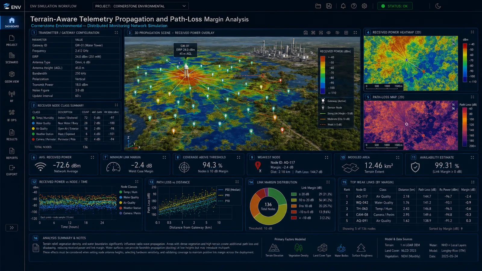
The propagation stage estimates received power and path loss between each sensor and the gateway or repeater serving it. It accounts for terrain elevation, vegetation density, water surfaces, industrial obstructions, antenna height, transmit power, and receiver sensitivity. This is the first stage that produces a quantitative link budget rather than a geometric screening.

This stage answers whether each link has enough margin to be reliable across the operating envelope, where received power drops below the gateway sensitivity threshold, which links are at risk of dropout when conditions degrade, and how raising a gateway mast, repositioning a sensor, or adding a repeater would change the answer. It exposes the difference between a network that is geometrically connected and a network that is RF-reliable.

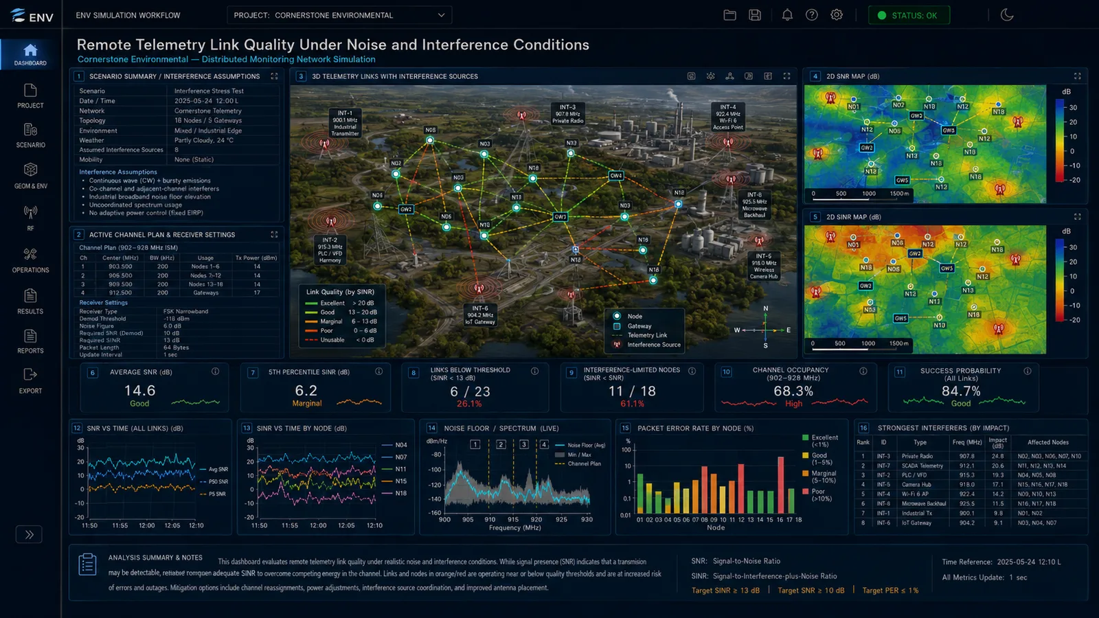
The interference stage layers a realistic noise and interference environment over the propagation model: ambient noise floor, nearby industrial RF sources, co-channel and adjacent-channel emissions, broadband noise from utility infrastructure, and any persistent or intermittent emitters in the operating area. SNR and SINR are evaluated per link, per node, and across the network.

This stage answers whether a link that looks strong on a coverage map will actually be reliable in operation, which nodes are interference-limited rather than coverage-limited, where channel reassignment or receiver retuning would recover margin, and which gateways need directional antennas, filtering, or relocation to clear a hostile receive environment.

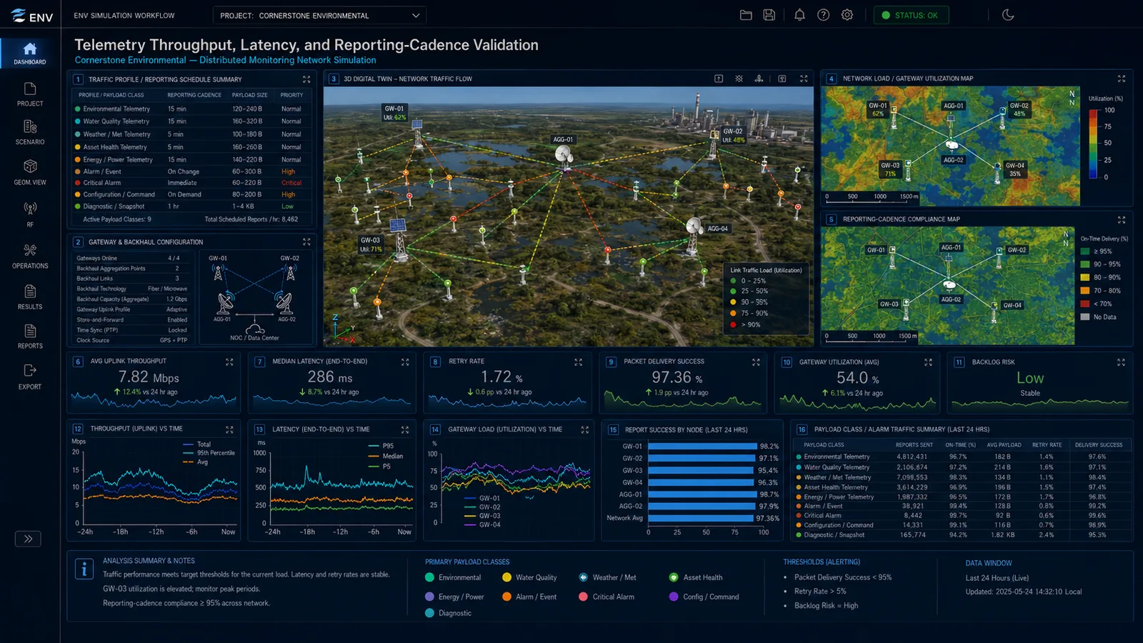
The throughput stage evaluates whether the network can support the required reporting cadence, payload size, alarm traffic, retry behavior, and gateway backhaul under realistic operating conditions. It models the full path from sensor uplink through gateway aggregation to the data backhaul.

This stage answers whether reporting intervals and payload sizes match available capacity, where latency or retry burden grows under load, which gateways are at risk of becoming a bottleneck, and how the network behaves when alarms collide with routine telemetry. It prevents the common failure mode where a deployment passes RF coverage checks but loses data or delays alarms because the operational data plane was never validated.

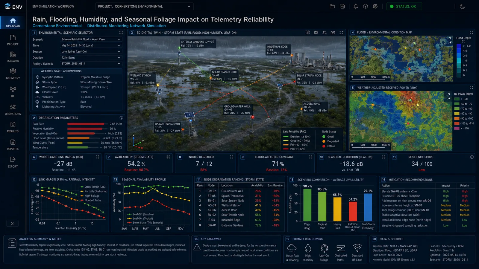
The environmental degradation stage evaluates the network under rain, storms, flooding, elevated humidity, water-level change, and seasonal foliage growth. It models how each of these conditions changes link margin, availability, and node accessibility.

This stage answers what link margin remains during heavy rain and storm conditions, which nodes are at risk of flood inundation or access loss, how leaf-on foliage seasonally degrades coverage, and where additional design margin, mast height, repeaters, or relocation are needed before the next high-risk season. It turns the network design from a fair-weather plan into one hardened for the conditions monitoring is actually meant to capture.

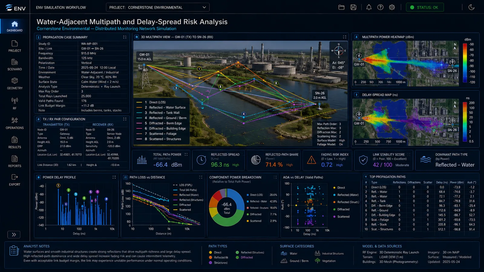
Remote environmental sites often combine smooth water surfaces with reflective industrial structures such as tanks, fences, berms, metal buildings, and elevated platforms. Each of these creates reflected and diffracted paths that arrive at the receiver after the direct signal, producing multipath fading and delay spread. The multipath stage uses 3D ray launching to identify direct, reflected, and diffracted contributions to each link and to quantify the resulting power and timing distribution.

This stage answers which links are dominated by reflected rather than direct energy, which links face wide delay spread and risk intermittent telemetry even at acceptable link budget, where antenna polarization, height, or relocation would reduce fading risk, and which links may need modulation or error-correction adjustments to remain stable.

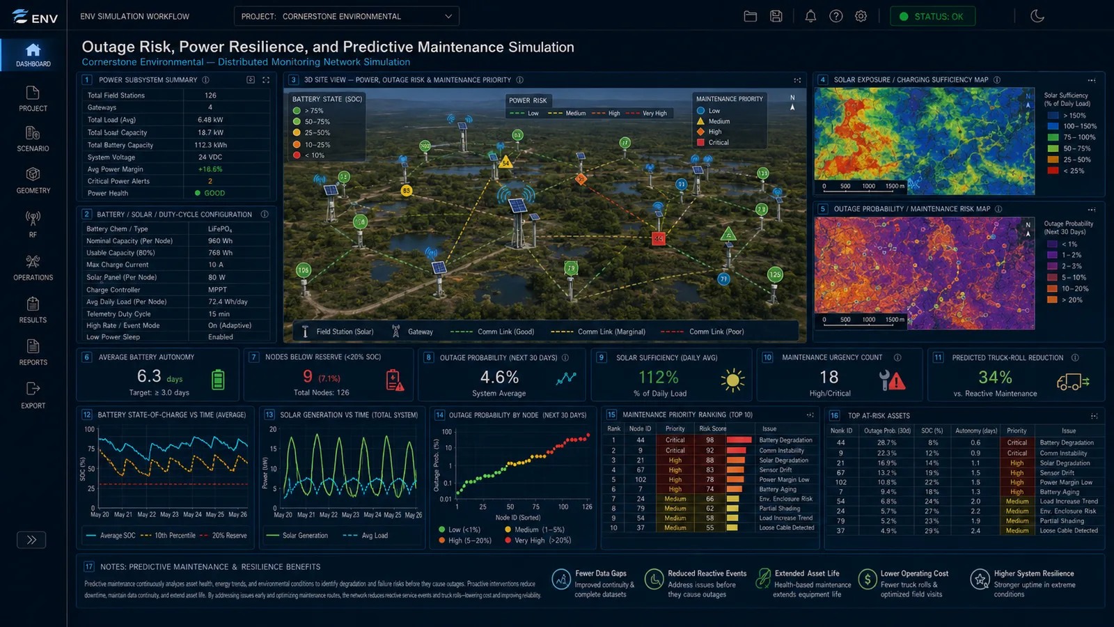
The outage stage models power state, solar sufficiency, battery autonomy, duty-cycle behavior, equipment aging, and the resulting outage probability across the network. It also estimates the operational benefit of proactive versus reactive maintenance routing.

This stage answers how many days of autonomy each node has under realistic conditions, which nodes are at risk of falling below reserve during low-solar windows, which assets are most likely to fail in the next maintenance interval, and how maintenance routes should be sequenced to reduce truck rolls while preventing data gaps. It connects technical design to operating cost: uptime, truck rolls, avoidable data loss, and equipment that fails before it is serviced.

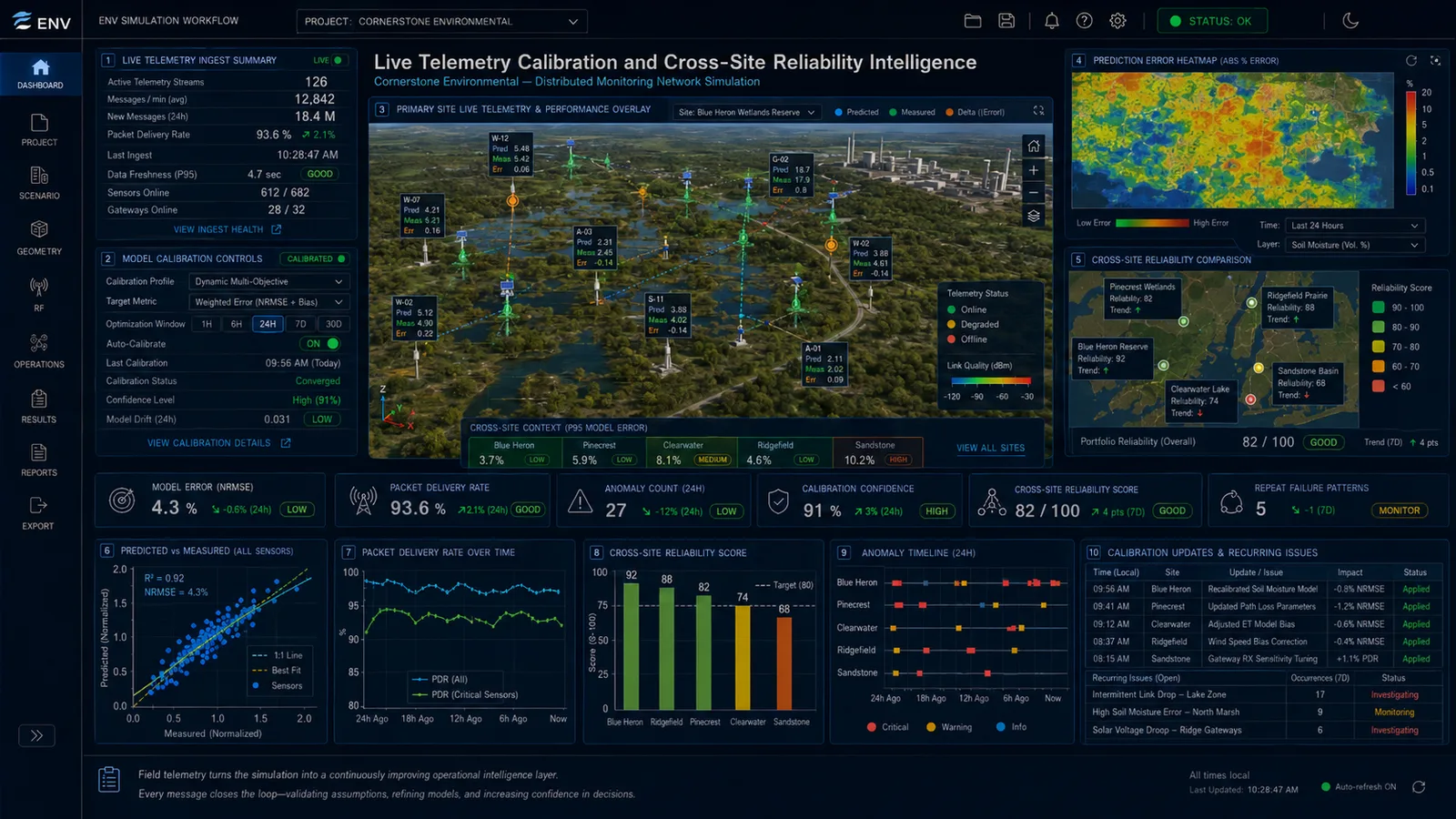
The telemetry feedback stage compares predicted performance against measured performance and uses the difference to recalibrate propagation, interference, throughput, and outage models. Inputs include live received signal strength, packet delivery rate, gateway logs, sensor health data, battery and solar telemetry, weather and water-level data, and maintenance records.

This stage answers how closely the model predicted real-world performance, where it was wrong and in what direction, which calibration updates are needed to make the next deployment more accurate, and which anomalies and repeat-failure patterns are emerging across the portfolio. Over time, it turns each site into structured knowledge that improves every later site.